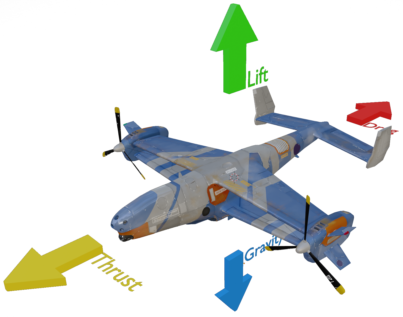
This flight model will be dealing with the four major forces of flight;
- Lift
- Drag
- Thrust
- Gravity
Units:
Force: Newtons
Mass: Kg
Speed: m/s
Area: m^2
Pressure: N/m2
Temperature: C
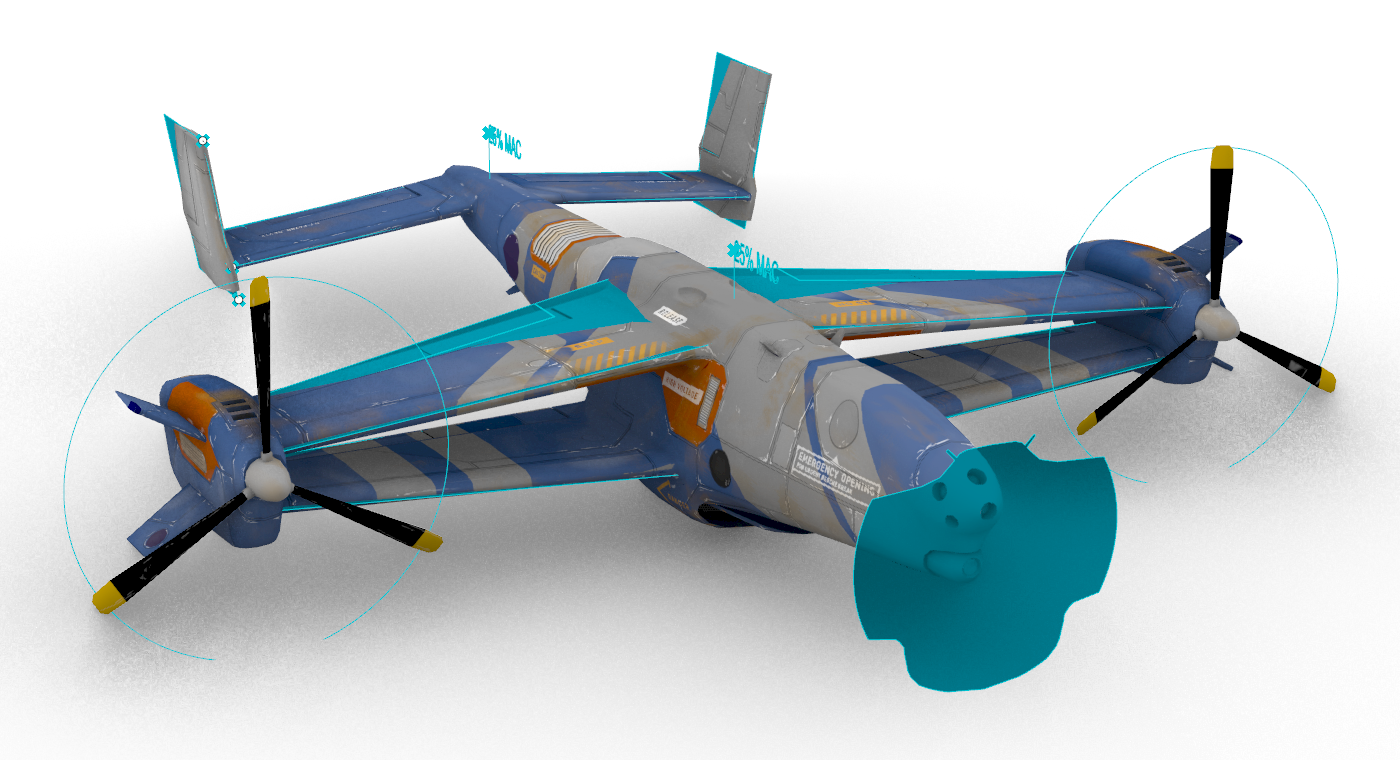
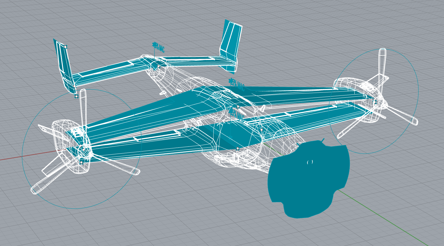
In this document we will deal with each in turn, starting with lift. Our flight model will be real-time, computing forces based on geometry defined in a static external JSON file. We will also develop our systems in a modular manner so that individual components can be upgraded separately over time. The graphic structure of an aircraft is displayed below. At the end of the article an example aircraft file will be dissected and discussed. Special thanks to Konstantin Predachenko, Aerospace Engineer from Ukraine for consulting on the specifics of aerodynamic theory.
Lift
It all starts with the lift equation;
L= CL(rV2/2)A
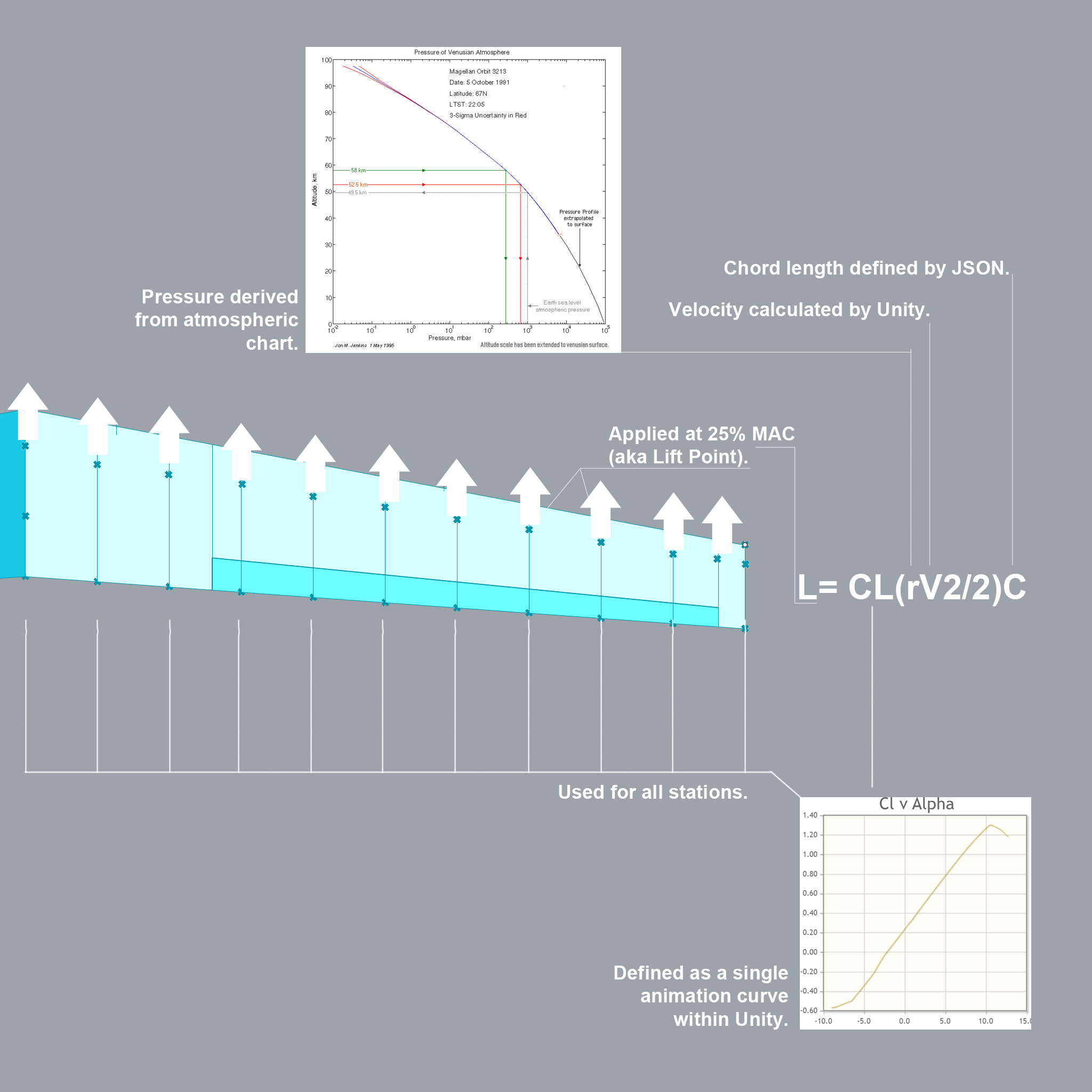
We will divide the variables of this equation into several subsystems. Cl, r and V^2 will be calculated dynamically as they depend on the aircraft’s state in space. C is a geometric property that will be defined in a static JSON file.
Cl: Coefficient of Lift
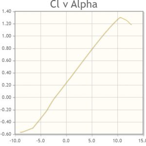
In this first iteration we will be using a single animation curve within Unity to define a notional airfoil for use throughout the whole simulation. This is because we will be replacing the animation curve with the Lifting Line Theory in the future.
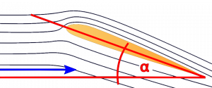
Once we replace it with LLT we will be defining each station using a static term: AoA0, or the AoA angle where no lift is developed.
r (rho): Atmospheric Pressure
This is a dynamic value. As we ascend in an atmosphere the pressure exerted by the molecules of that atmosphere diminishes as a function of the reduction in density over height.
It must be computed in real time because the aircraft will be ascending and descending and thus the pressure around it will change.
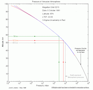
It is very important that this follows the Venusian atmospheric profile not just for simulation purposes but for gameplay as well. Venus has an extreme pressure gradient and it is an obstacle for player’s survival if they fly too low.
The pressure gradient is expressed in height above sea level (the surface) vs. pressure. In this graph, pressure is represented in millibar (mbar), though for sake of calculations it may be easier to use kg/m^2, in which case 1 mbar = 10.20 kg/m2.
We will need to know the height of the aircraft’s center of gravity (CoG) in km above the surface at all times. This value can then be applied to any attached lifting stations.
This chart should be modular, so that we can modify and swap it out in the future (perhaps with other planetary profiles). For now we can use a single animation curve and instantiate it in the beginning of the level. This should be part of the Planetary Profile.
Sidebar: Temperature
Future Looking:
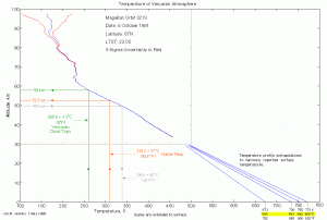
Another gameplay challenge will be Venus’s extreme temperature. For this reason we will need to track the aircraft’s height above the surface and apply it against a temperature gradient. This will affect the player’s health pool should they descend too low.
The aircraft’s maximum temperature will be defined in JSON. This does not need to be implemented now.
Graphs Courtesy of Shade Tree Physics.
V^2: Velocity
Unsurprisingly, this value must be computed in real-time. We will need to take the speed of each lift point and convert it to m/s in order to use it in the Lift Equation.
A: Area
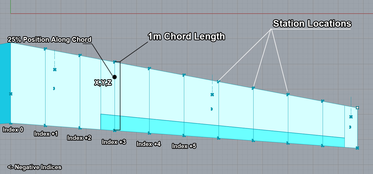
We will divide the wing into a number of stations within the JSON Aircraft Builder. For each station we will have the station index, the section area and the XYZ coordinates (in Unity’s coordinate system) of the point that is 25% of the length of the chord from the front of the wing.
Once we implement LLT, we will also include the 0 lift Angle of Attack for each station (AoA0). So we will need to allow for future properties within each station.
For each station we will run the Lift Calculation to generate a force at the 25% point. Each station’s velocity and angle of attack must be tracked independently. Each station is treated as it’s own “wing” for the purposes of the lift function.
Each station’s lift value (in Newtons) and vector will be applied as an individual force within Unity 3D.
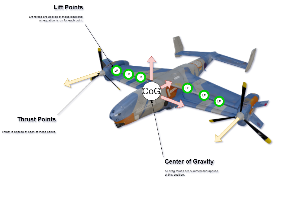
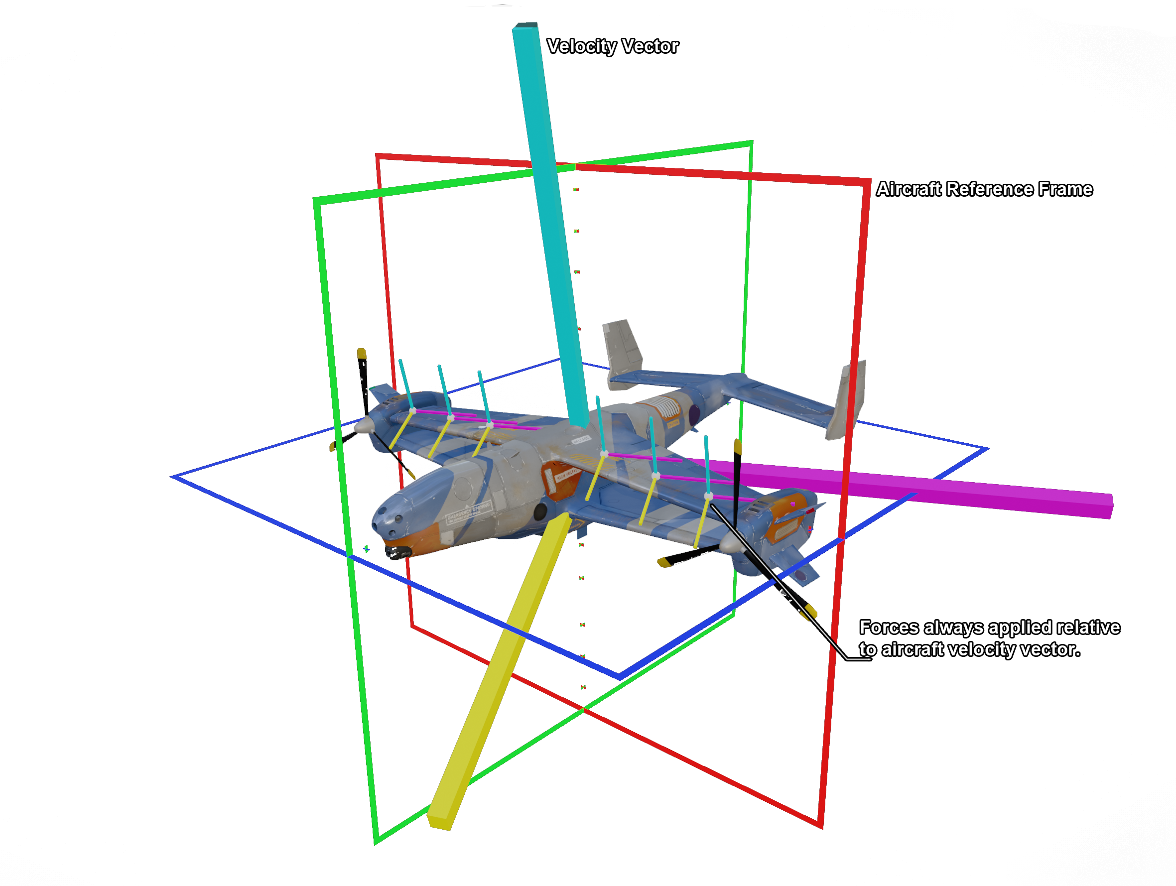
Lift is calculated per section taken from each wing. Each section has a length and at 25% of that length we create a “Lift Point”, which is a point force whose reference planes are aligned with the velocity vector of that point through space.
For each station we will run the lift calculation and then find the magnitude of that force. It will be applied at that location.
Known Limitations
The Cl of each station on a 3D wing cannot be accurately calculated by simply summing up the individual lift values of several 2D sections. For the sake of simplicity we will be using this method to get an initial prototype. However over time we will replace this calculation with a Cl calculated for each station determined with the Lifting Line Theory. This approach is able to create a coefficient of lift for each individual wing station, taking into account the influence of neighboring stations.
Drag
There are several equations we need to be concerned about when calculating drag.
Induced Drag, or drag that is generated by lift. This is calculated for and applied at each lifting point:
Cdi = (Cl^2) / (pi * AR * e)
In the case of a wing, we add Induced Drag to the Airfoil’s form drag to total Coefficient of Drag (Cdt):
Cdt = Cd + Cdi.
In the case of a fuselage body, we find the fuselage’s Cdt based on the Fineness Ratio of the fuselage:
Cd = (3*FR+4.5*(FR)^(-0.5)+21*(FR)^(-2))*Cf
Cf = (0.036/(Re)^(1/6))
Finally, the Drag Equation itself calculates Total Drag, which creates the force that directly opposes thrust:
D = Cdt * A * .5 *r * V^2
By summing the total drag of the aircraft we will create a point force at the aircraft’s center of gravity. The vector for this force will be opposite the direction of travel of the Center of Gravity, creating a force that opposes forward movement.
Drag Induced by Lift (Cdi)
Cdi = (Cl^2) / (pi * AR * e)
Cl: Coefficient of Lift
This is the same as the Cl referenced in “Lift”.
AR: Aspect Ratio
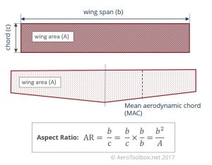
This is a static variable as it is defined by the aircraft’s geometry. It is available from the JSON file. The aspect ratio is the ratio between the wingspan and it’s averaged chord length (Mean Aerodynamic Chord).
Image credit: AeroToolbox
The efficiency factor is a nondimensional value. It will be calculated dynamically using LLT but for now it will be a static variable, defined per aircraft, available in the JSON.
Total Drag Coefficient (Wing)
Cdt = Cd + Cdi.
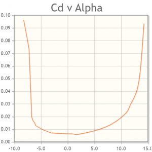
The total drag of a wing is calculated by taking the Form Drag (Cd) of the airfoil based on it’s Angle of Attack (chart to right) and adding it to the drag due to lift.
The Form Drag of the airfoil is a dynamic value, calculated based on the Lift Point’s orientation in space. Drag Induced by Lift is also a dynamic value, calculated by the previous equation.
Total Drag Coefficient (Fuselage)
Cd = (3*FR+4.5*(FR)^(-0.5)+21*(FR)^(-2))*Cf
Cf = (0.036/(Re)^(1/6))
The total drag of the Fuselage is calculated by finding it’s fineness ratio, length and cross sectional area. In the equation above:
FR: Fineness ratio: Static, defined in JSON as length/equivalent diameter (square root of (4xcross sectional area/pi)
Re: Dynamic, defined as: Length * Speed/Kinematic Viscosity (See equations below)
Length: Static, defined in JSON.
Viscosity is defined as Kinematic Viscosity. This is defined as Dynamic Viscosity / Density.
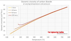
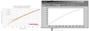
Since we know the Venusian atmosphere is 98% Carbon Dioxide, we can estimate the dynamic viscosity of the atmosphere using the chart to the right, showing the dynamic viscosity of CO2 over a range of temperatures.
Based on this graph, we have determined a constant for the density of the Venusian atmosphere;
Kinematic Viscosity = viscosity = (-1.6667e-05 x temperature^2+0.0483 x temperature+14) x (10e-6)/density (in kg / m ^ 3).
In this equation, Density and Temperature (in C) are dynamic variables that come from the atmospheric profile of Venus.
Total Drag: the Drag Equation
D = Cd * A * .5 *r * V^2
Coefficient of Drag
For definitions of Cd, see previous sections.
This value is defined by the Planet Profile and is the same as r used in other equations.
This is the velocity of the aircraft’s center of gravity and is the same as the other velocity measurements used throughout the software.
Thrust
In the interests of simplicity, thrust is a dynamic value that is defined by two static variables; a maximum thrust (in Newtons) and an XYZ value which indicates where the force should be applied. This will be expanded on later but is non-critical right now. These values can be accessed from the JSON. The dynamic variable is a 0-1 value from the minimum thrust to the maximum thrust, tied to the player’s throttle setting.
Gravity
The gravity of the planet is defined in the Planet Profile and is defined in m/s. It is a static value. It will be applied at the aircraft’s Center of Gravity and create a force that is point down towards the planet’s surface.
Aircraft Mass
The aircraft’s mass is a static value that is defined in the JSON file. However, the mass may be added to by attaching elements to the aircraft prefab, such as equipment or fuel tanks.
The aircraft’s Center of Gravity is defined as an XYZ coordinate in the JSON. For now, all aircraft will be assumed to be electric but we will add fuel tanks in the future.
Attachment hardpoints are static and defined as indexed XYZ coordinates in the JSON file.
Fuel tanks are defined in the same way, with a boolean indicating whether they can be filled and a variable saying how much they can carry. This is not necessary at the moment however.
The final Center of Gravity is a dynamic element that can be moved by adding additional elements to the aircraft in the scene.
Planetary Profile
The Planetary Profile is a JSON file which contains several static variables;
- The planet’s name.
- The gravity of the planet.
- The atmospheric pressure gradient.
- The temperature gradient.
Aircraft Header
In the aircraft header we find the aircraft’s name, which can be used for displaying the Aircraft Type on the targeting HUD.
Aircraft mass is the total mass in kg.
CoG Location is the XYZ coordinates in Unity space of the calculated center of gravity.
Fuselage area, length and fineness Ratio are the calculated values that can be used in the Fuselage Drag model.
Propulsion
In this section we are defining the location of the thrust points and the maximum thrust available for each engine.
Flying Surfaces
This is where the majority of the definitions are found. It is a list wings, defined by name. These wings are themselves lists of stations, each of which has a lift point, chord length and area.
This section also defines which stations are to be used as control surfaces and what type of control surfaces they can be used for.
At the moment we have five;
Ailerons: Controlling roll.
Elevators: Controlling pitch.
Rudders: Controlling yaw.
Flaps: Increasing wing lift/drag output.
None: Used when no control surface is present.
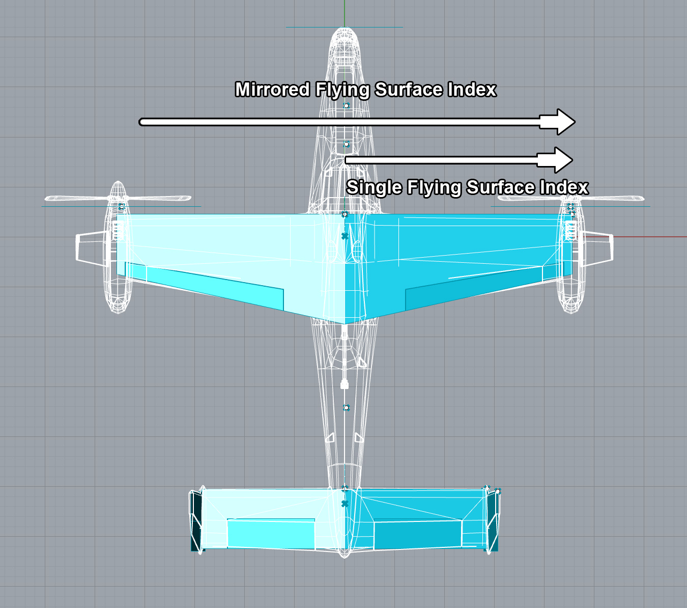
Each lift point is indexed from one to n. If a flying surface is mirrored (i.e. in a symmetrical wing) the values decrease from negative n to 1, then skip station 0 (as it has no area) and increase to positive n.
If a flying surface is not mirrored, i.e. in a horizontal tail, the lift points increase from 1 to n from root to tip.
For ease of use the wing stations in this example have been truncated to -3 and +3.
We first start with the “Flying Surfaces” section, which is the root list.
Then within that, we have the Wing Properties section, which defines the wing’s name, aspect ratio, what type of control surface it uses and a notional factor of how “clean” the wing is, defined as the wing’s Efficiency Factor.
From there, we get another sub-list, this one of lifting points.
Within this section, we get the lift point’s index, the area of the associated section, the chord length of that wing station, whether or not it should be used as a control surface and where the lift point is located in Unity XYZ space.
